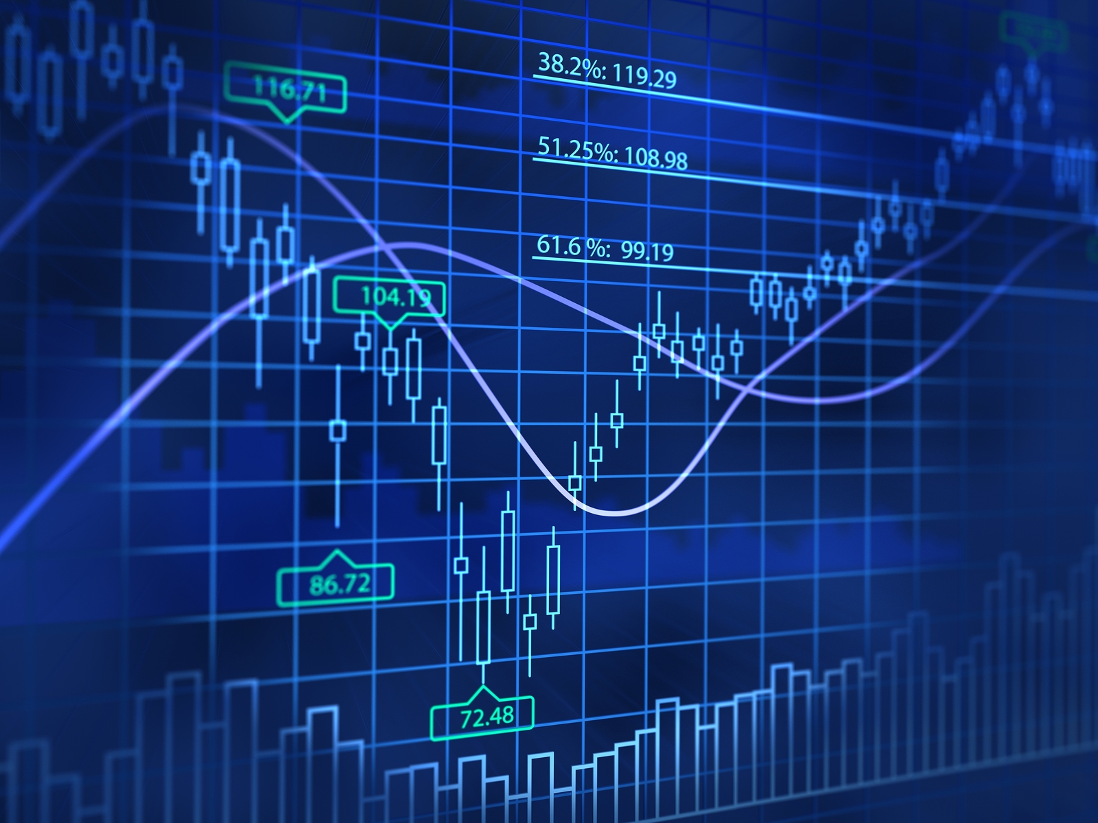
Subplot 기능을 활용하여 캔들차트와 보조지표(MACD) 출력하기
Subplot 기능을 활용하여 캔들차트와 보조지표(MACD) 출력하기
by JunPyo Park
Part of the Alpha Square Lecture Series:
오늘은 matplotlib의 subplot 기능을 활용하여 캔들차트와 MACD 같은 보조지표를 같이 그리는 방법에 대해 알아보도록 하겠습니다. 주피터 노트북 상에서 주가 데이터를 읽어와 캔들차트와 이동평균선을 그리는 방법, MACD에 대한 설명은 위의 링크를 참조해 주세요.
1. 주가 데이터를 읽어와 MACD 계산하기
주가 데이터를 읽어와 내용물을 확인합니다.
import pandas as pd
import pandas_datareader.data as web
from datetime import datetime

f = web.DataReader('AAPL', 'robinhood')
data = f.loc['AAPL']['2018-01':'2018-09']
data.head()
data.tail()
인덱스에 들어가 있는 날짜들의 타입을 문자열로 바꾸어 줍니다.
index = data.index.astype('str')
print("Period from ", index[0], " To ", index[-1])
5일 이동평균선과 20일 이동평균선을 계산하여 저장합니다.
ma5 = data['close_price'].rolling(window=5).mean()
ma20 = data['close_price'].rolling(window=20).mean()
MACD를 계산하도록 하겠습니다. MACD에 대한 설명은 기술적 분석 시리즈 #5 : MACD를 참고해 주세요. 기본적으로 MACD는 다음과 같이 계산됩니다.

MACD는 단순이동평균이 아닌 지수이동평균(Exponential Moving Average : EMA)을 사용합니다. 지수이동평균은 가중치를 부여한 평균의 일종으로써 최근의 데이터에 좀 더 가중치를 두는 방식입니다. 식을 전개했을 때 가중치를 살펴보면 k라는 평활 상수(smoothing constant)가 지수함수의 형태로 나타나기에 지수이동평균이라고 불립니다. 지수이동평균은 다음과 같은 코드를 통해 함수화할 수 있습니다.
def EMA(close, timeperiod):  # Exponential Moving Average : 지수이동평균
    k = 2/(1+timeperiod) # k : smoothing constant
    close = close.dropna()
    ema = pd.Series(index=close.index)
    ema[timeperiod-1] = close.iloc[0:timeperiod].sum() / timeperiod
    for i in range(timeperiod,len(close)):
        ema[i] = close[i]*k + ema[i-1] * (1-k)
    return ema
위의 지수이동평균 함수를 활용하여 다음과 같이 MACD 함수를 만들 수 있습니다. 12, 26, 9의 기간이 MACD를 산출하는데 보통 사용되기에 초깃값으로 지정해 두었습니다. 물론 차트 분석가의 재량에 따라 다른 값을 사용할 수 있습니다. 이런 경우에는 파라미터에 다른 값을 넘겨 주면 됩니다.
def MACD(close, fastperiod=12, slowperiod=26, signalperiod=9):
    macd = EMA(close, fastperiod) - EMA(close, slowperiod)
    macd_signal = EMA(macd, signalperiod)
    macd_osc = macd - macd_signal
    df = pd.concat([macd, macd_signal, macd_osc],axis=1)
    df.columns = ['MACD','Signal','Oscillator']
    return df
위에서 추출한 종가 데이터가 소숫점(.)이 들어간 포맷팅 때문에 문자열 타입을 가지고 있습니다. 이를 소수점 자료형(float)으로 바꾸어 줍니다.
close_price = data['close_price'].astype(float)
다음과 같이 만들어둔 함수를 통해 MACD와 시그널 오실레이터를 얻을 수 있습니다.
macd = MACD(close_price)
macd.tail()
2. subplot 기능 활용하기
여러 개의 차트를 레이아웃에 맞추어 그려야 할 때 matplotlib에서 제공하는 subplot 기능을 활용할 수 있습니다. 여기서는 subplot2grid를 활용하도록 하겠습니다. 예제를 하나 살펴보도록 하겠습니다.
import matplotlib.pyplot as plt

plt.close('all')
fig = plt.figure(figsize=(9,9))

ax1 = plt.subplot2grid((3, 3), (0, 0))
ax2 = plt.subplot2grid((3, 3), (0, 1), colspan=2)
ax3 = plt.subplot2grid((3, 3), (1, 0), colspan=2, rowspan=2)
ax4 = plt.subplot2grid((3, 3), (1, 2), rowspan=2)

plt.tight_layout()

제각기 다른 사이즈의 차트 4개가 생성되었는데 다음 그림과 같이 각 차트 왼쪽 위 꼭짓점을 좌표에 대응 시켜보면 코드 이해가 한결 쉬워집니다.


코드 마지막 부분에 있는 plt.tight_layout() 명령어는 차트끼리 충돌하는 것을 막아주는 명령어입니다.
3. 캔들차트와 보조지표 plot 하기
이제 위 내용들을 바탕으로 최종 차트를 그려보도록 하겠습니다. 전체 코드는 다음과 같습니다. 파이썬에서 캔들차트와 이동평균선 그리기를 먼저 완료한 뒤 진행 하시면 쉽게 따라하실 수 있습니다.
from mpl_finance import candlestick2_ohlc
import matplotlib.pyplot as plt
%matplotlib inline
import matplotlib.ticker as ticker
import numpy as np

# 차트 레이아웃을 설정합니다.
fig = plt.figure(figsize=(12,10))
ax_main = plt.subplot2grid((5, 1), (0, 0), rowspan=3)
ax_sub = plt.subplot2grid((5, 1), (3, 0))
ax_sub2 = plt.subplot2grid((5, 1), (4, 0))

# 메인차트를 그립니다.
ax_main.set_title('Apple Inc. Q1~Q3 2018 Stock Price',fontsize=20)
ax_main.plot(index, ma5, label='MA5')
ax_main.plot(index, ma20, label='MA20')
candlestick2_ohlc(ax_main,data['open_price'],data['high_price'],
                  data['low_price'],data['close_price'],width=0.6)

ax_main.legend(loc=5)

# 아래는 날짜 인덱싱을 위한 함수 입니다.
def mydate(x,pos):
    try:
        return index[int(x-0.5)]
    except IndexError:
        return ''

# ax_sub 에 MACD 지표를 출력합니다.
ax_sub.set_title('MACD',fontsize=15)
macd['MACD'].iloc[0] = 0
ax_sub.plot(index,macd['MACD'], label='MACD')
ax_sub.plot(index,macd['Signal'], label='MACD Signal')
ax_sub.legend(loc=2)

# ax_sub2 에 MACD 오실레이터를 bar 차트로 출력합니다.
ax_sub2.set_title('MACD Oscillator',fontsize=15)
oscillator = macd['Oscillator']
oscillator.iloc[0] = 1e-16
ax_sub2.bar(list(index),list(oscillator.where(oscillator > 0)), 0.7)
ax_sub2.bar(list(index),list(oscillator.where(oscillator < 0)), 0.7)

# x 축을 조정합니다.
ax_main.xaxis.set_major_locator(ticker.MaxNLocator(7))
ax_main.xaxis.set_major_formatter(ticker.FuncFormatter(mydate))
ax_sub.xaxis.set_major_locator(ticker.MaxNLocator(7))
ax_sub2.xaxis.set_major_locator(ticker.MaxNLocator(7))
fig.autofmt_xdate()

# 차트끼리 충돌을 방지합니다.
plt.tight_layout()
plt.show()
