Pyod 사용해보기

Table of Contents

• 1  모듈 불러오기
• 2  데이터 생성
• 3  모델 피팅
• 4  Evaluation
• 5  시각화

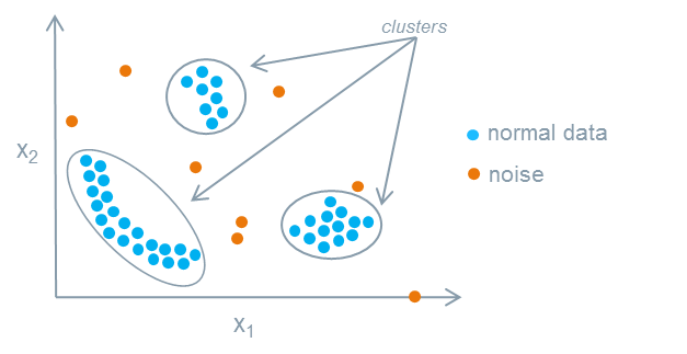
PyOD is a comprehensive and scalable Python toolkit for detecting outlying objects in multivariate data. This exciting yet challenging field is commonly referred as Outlier Detection or Anomaly Detection.

아웃라이어나 아노말리(이상치) 탐지를 위해 만들어진 모듈

201110 기준 Numpy==1.19.4 에서 에러남, Numpy==1.19.3 버젼 에서 실행됨

모듈 불러오기

from pyod.utils.example import visualize
from pyod.utils.data import evaluate_print
from pyod.utils.data import generate_data
from pyod.models.knn import KNN

contamination = 0.1  # percentage of outliers
n_train = 200  # number of training points
n_test = 100  # number of testing points

데이터 생성

# Generate sample data
X_train, y_train, X_test, y_test = \
    generate_data(n_train=n_train,
                  n_test=n_test,
                  n_features=2,
                  contamination=contamination,
                  random_state=42)

c:\users\wnsvy\miniconda3\envs\pyod\lib\site-packages\pyod\utils\data.py:190: FutureWarning: behaviour="old" is deprecated and will be removed in version 0.8.0. Please use behaviour="new", which makes the returned datasets in the order of X_train, X_test, y_train, y_test.
  FutureWarning)

X_train.shape, y_train.shape

((200, 2), (200,))

X_test.shape, y_test.shape

((100, 2), (100,))

모델 피팅

clf_name = 'KNN'
clf = KNN()
clf.fit(X_train)

KNN(algorithm='auto', contamination=0.1, leaf_size=30, method='largest',
  metric='minkowski', metric_params=None, n_jobs=1, n_neighbors=5, p=2,
  radius=1.0)

# 예측된 결과
clf.labels_

array([0, 0, 0, 0, 0, 0, 0, 0, 0, 0, 0, 0, 0, 0, 0, 0, 0, 0, 0, 0, 0, 0,
       0, 0, 0, 0, 0, 0, 0, 0, 0, 0, 0, 0, 0, 0, 0, 0, 0, 0, 0, 0, 0, 0,
       0, 0, 0, 0, 0, 0, 0, 0, 0, 0, 1, 0, 0, 0, 0, 0, 0, 0, 0, 0, 0, 0,
       0, 0, 0, 0, 0, 0, 0, 0, 0, 0, 0, 0, 0, 0, 0, 0, 0, 0, 0, 0, 0, 0,
       0, 0, 0, 0, 0, 0, 0, 0, 0, 0, 0, 0, 0, 0, 0, 0, 0, 0, 0, 0, 0, 0,
       0, 0, 0, 0, 0, 0, 0, 0, 0, 0, 0, 0, 0, 0, 0, 0, 0, 0, 0, 0, 0, 0,
       0, 0, 0, 0, 0, 0, 0, 0, 0, 0, 0, 0, 0, 0, 0, 0, 0, 0, 0, 0, 0, 0,
       0, 0, 0, 0, 0, 0, 0, 0, 0, 0, 0, 0, 0, 0, 0, 0, 0, 0, 0, 0, 0, 0,
       0, 0, 0, 0, 1, 1, 1, 1, 1, 1, 1, 1, 1, 1, 0, 1, 1, 1, 1, 1, 1, 1,
       1, 1])

Evaluation

y_train_pred = clf.labels_
y_train_scores = clf.decision_scores_

y_test_pred = clf.predict(X_test)
y_test_scores = clf.decision_function(X_test)

print("On Training Data:")
evaluate_print(clf_name, y_train, y_train_scores)

print("\nOn Test Data:")
evaluate_print(clf_name, y_test, y_test_scores)

On Training Data:
KNN ROC:0.9992, precision @ rank n:0.95

On Test Data:
KNN ROC:1.0, precision @ rank n:1.0

시각화

# visualize the results
visualize(clf_name, X_train, y_train, X_test, y_test, y_train_pred,
          y_test_pred, show_figure=True, save_figure=True)